In this post we will look at path space measures over continuous time Markov chain (CTMC) paths. This description is taken from a paper I co-authored arXiv 2402.04997 Appendix C which follows the exposition in Stochastic Processes: From Applications to Theory by Del Moral and Penev Chapter 18. This is a topic I found difficult to find an intuitive explanation of when I first started and so I hope this post can be useful to others.

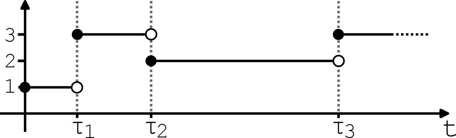
A path of a CTMC is a single trajectory from time \(0\) to time \(t\). The trajectory is a function \(\omega : s \in [0, t] \mapsto \omega_s \in \{1, \dots , S \}\) that is everywhere right continuous and has left limits everywhere (also known as càdlàg paths). Intuitively, it is a function that takes in a time variable and outputs the position of the particle following the trajectory at that time. The càdlàg condition in our case states that at jump time \(\tau\) we have \(\omega_\tau\) taking the new jumped to value and \(\omega_{\tau}^- := \lim_{s \uparrow \tau} \omega_s\) being the previous value before the jump.

\[ \begin{aligned} \mathbb{P}(W \in \mathrm{d} \omega) := \mathbb{P} \left( W_0 \in \mathrm{d} \omega_{0}, (T_1, W_{T_1}) \in \mathrm{d} (t_1, \omega_{t_1}), \dots (T_n, W_{T_n}) \in \mathrm{d} (t_n, \omega_{t_n}), T_{n+1} \geq t \right) \end{aligned} \]

where \(\mathrm{d} \omega_{t_n}\) and \(\mathrm{d} t_n\) denote infinitesimal neighborhoods around the points \(\omega_{t_n} \in \{1, \dots, S \}\) and \(t_n \in [0, t]\). This is the same sense in which a probability density function assigns probabilities to the infinitesimal neighborhood around a continuous valued variable.

Our goal is to find an expression for \(\mathbb{P}(W \in \mathrm{d} \omega) \) in terms of known quantities that describe the CTMC i.e. the rate matrix. We can start by splitting \(\mathbb{P}(W \in \mathrm{d} \omega) \) into a product of conditional factors

\[ \begin{aligned} \mathbb{P}(W \in \mathrm{d} \omega) = &\mathbb{P}(W_0 \in \mathrm{d} \omega_0) \mathbb{P}((T_1, W_{T_1} \in \mathrm{d} (t_1, \omega_{t_1}) | W_0) \times \dots \\ &\times \mathbb{P}((T_n, W_{T_n}) \in \mathrm{d} (t_n, \omega_{t_n}) | W_0, (T_1, W_{T_1}), \dots, (T_{n-1}, W_{T_{n-1}})) \\ &\times \mathbb{P}(T_{n+1} \geq t | W_0, (T_1, W_{T_1}), \dots, (T_{n}, W_{T_{n}})) \end{aligned} \]\[ \begin{align} \mathbb{P}(W \in \mathrm{d} \omega) = &\mathbb{P}(W_0 \in \mathrm{d} \omega_0) \times \label{factor1} \\ &\mathbb{P}(T_1 \in \mathrm{d} t_1 | W_0) \times \label{factor2} \\ &\mathbb{P}(W_{T_1} \in \mathrm{d} \omega_{t_1} | W_0, T_1, W^{-}_{T_1} = W_0) \times \label{factor3}\\ &\dots \times \\ &\mathbb{P}(T_n \in \mathrm{d} t_n | W_0, (T_1, W_{T_1}), \dots, (T_{n-1}, W_{T_{n-1}})) \times \\ &\mathbb{P}(W_{T_n} \in \mathrm{d} \omega_{t_n} | W_0, (T_1, W_{T_1}), \dots, T_n, W^{-}_{T_{n}} = W_{T_{n-1}}) \times \\ &\mathbb{P}(T_{n+1} \geq t | W_0, (T_1, W_{T_1}), \dots, (T_{n}, W_{T_{n}})) \label{factor4} \end{align} \]

We have split \(\mathbb{P}(W \in \mathrm{d} \omega) \) into individual probabilities for all the events that make a \(W \) path unique. We consider paths of time length \( t \). During this time we index all the jumps as \( 1 \) to \( n \). It starts with the probability that the initial state is in a certain position (Eq. \ref{factor1}). We then have the probability that the first waiting time is in local neighborhood \( \mathrm{d} t_1 \) (Eq. \ref{factor2}). This is followed by the probability that the particle jumps to new state \(W_{T_1} \) that is in local neighborhood \( \mathrm{d} \omega_{t_1}\) (Eq. \ref{factor3}). This is conditioned on the fact that the left limit \( W_{T_1}^-\) is still in the previous state \(W_0 \) because we know the jump time is \(T_1\). These factors are repeated for all times up to \(T_n \) with the conditioning growing as more history of the CTMC path is built up.

The final aspect of a CTMC path \(W \) that we need to assign probability to is that if we are looking at paths of time length \( t\), then we need particle to wait in the final position until the end of time window. Otherwise, if it jumped before reaching time \( t \), then this wouldn’t be the final state by definition! We therefore need to include the probability that the particle will wait in this final position (Eq. \ref{factor4}).

For discrete state spaces \( \mathbb{P}(W_{T_n} \in \mathrm{d} \omega_{t_n}) \) is simply \(\mathbb{P}(W_{T_n} = \omega_{t_n})\) because we use the discrete measure. We also note that for CTMCs, the markov property ensures the probability of a jump does not depend on the entire history but only on the previous state. This gives

\[ \begin{aligned} \mathbb{P}(W \in \mathrm{d} \omega) = &\mathbb{P}(W_0 = \omega_0) \times \\ &\mathbb{P}(T_1 \in \mathrm{d} t_1 | W_0) \times \\ &\mathbb{P}(W_{T_1} = \omega_{t_1} | T_1, W^{-}_{T_1} = W_0) \times\\ &\dots \times \\ &\mathbb{P}(T_n \in \mathrm{d} t_n | T_{n-1}, W_{T_{n-1}}) \times \\ &\mathbb{P}(W_{T_n} = \omega_{t_n} | T_n, W^-_{T_n} = W_{T_{n-1}}) \times \\ &\mathbb{P}(T_{n+1} \geq t | T_n, W_{T_{n}}) \end{aligned} \]

In these factors, we still need to condition on the previous jump time because we need to know a jump occurs. It is now left to us to work out the forms for each of these factors.

We start by reminding ourselves of the definition of a CTMC with rate matrix \(R_t\). The CTMC waits in the current state for an amount of time determined by an exponential random variable with time-inhomogeneous rate \(R_t(W_t) := \sum_{k \neq W_t} R_t(W_t, k)\), see [1] and [2] Appendix A for more details. After the wait time is finished, the CTMC jumps to a next chosen state where the jump distribution is

\[ \begin{equation*} \mathbb{P}(W_{t_k} | W_{t_k}^-) = \frac{R_t(W_{t_k}^-, W_{t_k}) \left(1 - \delta \{W_{t_k}^- = W_{t_k} \} \right) } { R_t(W_{t_k}^-) } \end{equation*} \]

From this definition, we immediately get that

\[ \begin{equation*} \mathbb{P}(W_{T_n} = \omega_{t_n} | T_n, W^-_{T_n} = W_{T_{n-1}}) = \frac{R_{T_n}(W_{T_n}^-, W_{T_n}) } { R_{T_n}(W_{T_n}^-) } \end{equation*} \]

Note that we automatically have \(\delta \{ W_{T_n}^- = W_{T_n} \} = 0\) because we condition on the fact a jump occurs at \(T_n \) and a jump necessitates a change in value by definition.

Now we can work on the time related quantities. For an exponential random variable with time-inhomogeneous rate, the cumulative distribution function is given by

\[ \begin{equation*} \mathbb{P}(T < t) = 1 - \exp \left( - \int_{s=0}^{s=t} R_s(W_s^-) \mathrm{d} s \right) \end{equation*} \]

Therefore, the probability density function, \(p(t) = \frac{\partial}{\partial t} \mathbb{P}(T < t)\), is

\[ \begin{equation*} p(t) = \exp \left( - \int_{s=0}^{s=t} R_s(W_s^-) \mathrm{d} s \right)R_t(W_t^-) \end{equation*} \]

From this we get that

\[ \mathbb{P}(T_n \in \mathrm{d} t_n | T_{n-1}, W_{T_{n-1}}) = \exp \left( - \int_{s=T_{n-1}}^{s=T_n} R_s(W_s^-) \mathrm{d} s \right) R_{T_n}(W_{T_n}^-) \mathrm{d} t_n \]

We finally note that if we wish to know \(\mathbb{P}(T_k < t | T_{k-1})\) i.e. the probability that the \(k\)-th jump time is less than \(t\) given we know the \(k-1\)-th jump time, then this is just an exponential random variable started at time \(T_{k-1}\) when the previous jump occurred,

\[ \begin{equation*} \mathbb{P}(T_k < t | T_{k-1}) = 1 - \exp \left( - \int_{s=T_{k-1}}^{s=t} R_s(W_s^-) \mathrm{d} s \right) \end{equation*} \]

In other words, we simply start a new exponential timer once the previous jump occurs and the same equation carries through. Therefore we have

\[ \mathbb{P}(T_{n+1} \geq t | T_n, W_{T_{n}}) = \exp \left( - \int_{s=T_{n}}^{s=t} R_s(W_s^-) \mathrm{d} s \right) \]

We now substitute all these factors into our equation for \(\mathbb{P}( W \in \mathrm{d} \omega )\).

\[ \begin{aligned} \mathbb{P}(W \in \mathrm{d} \omega) =& p_0(W_0) \times \\ & \exp \left( - \int_{s=0}^{s=T_1} R_s(W_s^-) \mathrm{d} s \right) R_{T_1}(W_{T_1}^-) \mathrm{d} t_1 \times \\ & \frac{R_{T_1}(W_{T_1}^-, W_{T_1})}{R_{T_1}(W_{T_1}^-)} \times \\ & \dots \times\\ & \exp \left( - \int_{s=T_{n-1}}^{s=T_n} R_s(W_s^-) \mathrm{d} s \right) R_{T_n}(W_{T_n}^-) \mathrm{d} t_n \times \\ & \frac{R_{T_n}(W_{T_n^-}, W_{T_n})}{R_{T_n}(W_{T_n}^-)} \times \\ & \exp \left( - \int_{s=T_n}^{s=t} R_s(W_s^-) \mathrm{d} s \right) \end{aligned} \]

where \(p_0(W_0) \) is some initial discrete distribution for the start point of the trajectory. There are a lot of cancellations and combining all the exponential terms, we get

\[ \begin{aligned} \mathbb{P}(W \in \mathrm{d} \omega) &= p_0(W_0) \exp \left( - \int_{s=0}^{s=t} R_s(W_s^-) \mathrm{d} s\right) \prod_{k=1}^n R_{T_k}(W_{T_k}^-, W_{T_k}) \mathrm{d} t_k\\ &= p_0(W_0) \exp \left( - \int_{s=0}^{s=t} R_s(W_s^-) \mathrm{d} s\right) \prod_{s:W_s \neq W_s^-} R_{s}(W_{s}^-, W_{s}) \mathrm{d} s \end{aligned} \]

This path space measure is useful for understanding Girsanov’s transformation for CTMCs. Girsanov’s transformation can be thought of as `importance sampling’ for path space measures. Specifically, if we take an expectation with respect to path measure \(\mathbb{P}\), \(\mathbb{E}_{\mathbb{P}} \left[f (W) \right]\), then this is equal to \(\mathbb{E}_{\mathbb{Q}} \left[f(W) \frac{\mathrm{d} \mathbb{P}}{\mathrm{d} \mathbb{Q}}(W) \right]\) where \(\mathbb{Q}\) is a different path measure and \(\frac{\mathrm{d} \mathbb{P}}{ \mathrm{d} \mathbb{Q}}\) is known as the Radon-Nikodym derivative. The path measure \(\mathbb{Q}\) will result from considering a CTMC with a different rate matrix to our original measure \(\mathbb{P}\). Girsanov’s transformation allows us to calculate the expectation which should have been taken with respect to the CTMC with \(\mathbb{P}\) rate matrix instead with a CTMC with rate matrix corresponding to \(\mathbb{Q}\).

The Radon-Nikodym derivative in our case has a form that is simply the ratio of \(\mathbb{P}(W \in \mathrm{d} \omega)\) and \(\mathbb{Q}(W \in \mathrm{d} \omega)\). Let \(R_t\), \(p_0\) be the rate matrix and initial distribution defining \(\mathbb{P}\) and let \(R_t'\), \(p'_0\) be the rate matrix and initial distribution defining \(\mathbb{Q}\).

\[ \begin{equation*} \frac{\mathrm{d} \mathbb{P}}{\mathrm{d} \mathbb{Q}} (W) = \frac{ p_0(W_0) \exp \left( - \int_{s=0}^{s=t} R_s(W_s^-) \mathrm{d} s \right) \prod_{s: W_s \neq W_s^-} R_s(W_s^-, W_s) } { p'_0(W_0) \exp \left( - \int_{s=0}^{s=t} R'_s(W_s^-) \mathrm{d} s \right) \prod_{s: W_s \neq W_s^-} R'_s(W_s^-, W_s) } \end{equation*} \]

References #

[1] Norris, J. R. Markov chains. Cambridge university press, 1998

[2] Campbell, A., Benton, J., De Bortoli, V., Rainforth, T., Deligiannidis, G., and Doucet, A. A continuous time framework for discrete denoising models. Advances in Neural Information Processing Systems, 2022